                  ______
                 /      |       ________
                /       |____  /        \
               /        |    \/   _      \
               \       ___       /_\      \
                \      \_/          .      \
                 \          /\_____/       /
                  \________/      |       /
                                  |______/
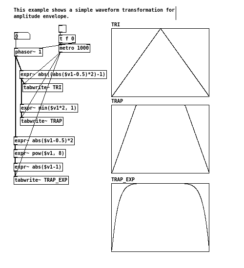
Some wave forms, like sawtooth, are easy to implement and provides useful building blocks in signal manipulation. Trapezoid is another such example.
It is particularly suitable used as amplitude envelope, in which smooth attack and decay can be guaranteed, whilst the “on” portion of the envelope stays fully open for as long as possible. For instance, if an triangle wave had been used, the envelope will never stay fully open, as the signal starts to ramp down as soon as it reaches the top. As a result, modulated signal can appear to be continuously fading in and out, or the lost of overall “loudness”. Trapezoid, on the other hand, provides an convenient method to address these issues.
Trapezoid, in fact, can be easily constructed out of a triangle wave, with two additional operates involved. The triangle is first scaled up (multiplication) by a desirable amount, and than clipped(min()) at the maximum y-axis value of the envelope, which conventionally is 1. The more the signal is scaled, the steeper the sides of the resulting trapezoid becomes, thus shorter in attack/decay duration.
One other variation would be to use the pow() function, turning the liner slopes of the (inverted) triangle into exponential curves. The envelope is then flipped over to the right orientation for use. The advantage of this method is that, given the same breakpoint locations, the total “on” area of the signal would be larger than that of the linear trapezoid. The resulting modulation would have even less perceived loudness loss. However, such a shape resembles more of a classic jello than a trapezoid.
In the previous post on sample play back, where a given sound file are splitted into multiple sections, clipping can often occur at the edges of the segments due to non zero-crossing. This is an ideal scenario to apply trapezoid, or equivalent variants, to rectify such error, by using it as a amplitude envelope.
Exercise:
- Are there other types of slops/curves that can be used in the waveform transformation similar to the exmple above?
-*-
Although the examples so far all uses simple sound synthesis to demonstrate the underlying principles of the signal-only methodology, they can easily be extended to control and manipulate audio samples as well.
As sound files are in essence arrays of values stored on disk, playing back an sample can be done simply by using a [phasor~] to systematically step through each of the values in the file.
To begin with, one must know the length of the chosen file, in number of samples. This value can be obtained from the output of the [soundfiler] object, and can then be multiplied with a sawtooth signal. The result is a complete indexing from the beginning to the end of the file, which the [tabread~] object can accept as input.
To resolve the “correct” rate for playback, however, can be somewhat ambiguous. On the one hand, there is the actual speed in which the sample was first recorded. On the other hand, there is the desired speed in which the current composition demands.
Assuming the goal is to playback at the recorded speed, the original sample rate also must be known. By dividing the length of the sound file with the sample rate, the time duration is therefore known, and can easily be converted into frequency.
The following example shows an simple playback setup
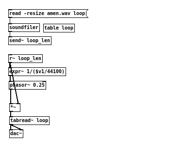
Such a result admittedly is not very interesting compositionally. However, by applying the principles that had been introduced previously, step counting for instance, one can easily make the necessary changes to give much more flexibility and possibilities.
This second example demonstrates the ability to slice the sample into definable sections, and rearrange them according to a modulated counter.
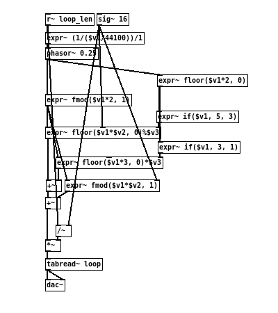
Note that there is no amplitude envelope in the above example to correct the hard clipping at the edges of each sample sections. To achieve this, one can produce an signal in the shape of (isosceles) trapezoid signal to modulate over the sample values.
Exercise:
- Besides the frequency, what other parameters can be modified/modulated for sample playback?
- Are there other interesting counting method to experiment with?
-*-
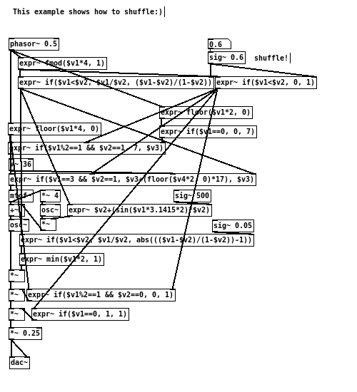
When creating subdivisions of time with fmod() and floor(), it would produce equal segments by default. This is often convenient for further processing, because the duration of each measures are identical. However, it may not always be so musically desirable to derive time intervals in such a uniformed manor. Often, a slight shuffle is intentionally introduced into repeating rhythmic patterns, so to prevent the end result from sounding too static. This is generally referred to as the “swing”.
To shuffle a sawtooth signal, the following method can be used:
   [phasor~ 0.5]                                 [sig~ 0.6]
   |                                             |
   [expr~ if($v1<$v2, $v1/$v2, ($v1-$v2)/(1-$v2))]
   |
   [s~ shuffled_signal]
The second inlet($v2) of the [expr~] signifies the amount, as well as the direction, of the shuffle. When set to 0.5, the input phasor would be divided equally, where as 0.6 would increase the duration of the first section, making it a little be longer than the second segment. Note that the allowed value for $v2, in this case, would be between 0 and 1.
Once a sawtooth signal can be halved in arbitrary proportion, it would also be useful to be able to identify the current position of the signal, in relation to the two uneven portions of the “swing”.
To to this, the following can be used in combination with the previous example.
   [phasor~ 0.5]           [sig~ 0.6]
   |                       |
   [expr~ if($v1<$v2, 0, 1)]
   |
   [s~ shuffle_idx]
In this case, the two sections can now be identified with an index value of 0 and 1. It is worth noting that, with shuffled signal, it would be more difficult to obtain a counting signal from it using floor(). If a specific segment of the shuffled signal needs to be isolated within a larger musical phrase, for example, a combination of normal floor() counter and the above mentioned indexing can be used to achieve that. This can be seen in the example patch below.
The musical effect in which shuffling creates is very much similar to syncopation. By intentionally distributing the time units unevenly, an off-beat “groove” sensation can be perceived from it. However, with syncopated rhythms, the amount of “shuffle” would still fall into the evenly divided time subdivisions. With shuffling, on the other hand, would usually be a adjustable amount (as found in many drum machine), usually a percentage of the current time unit/measurement. For example, given two consecutive 4 quarter notes, a swing of 10% can be set, so that the first beat are slightly longer than the second.
-*-
Previously, the fmod() function had been used in the context of frequency multiplication. For example:
[phasor~ 0.25] -> [expr~ fmod($v1*4, 1)]
Besides this, it can also be used to shift the phase position of a sawtooth oscillator. The principle is largely the same as the example above, apart from replacing the multiplication with addition, which represents the amount of displacement. For example:
[phasor~ 0.25] -> [expr~ fmod($v1+(1/4.0), 1)]
This will push the phase position of the input sawtooth by a quarter of the total wavelength.
                                             Original phase position
     .    /|       /|       /|       /|
     .   / |      / |      / |      / |
     .  /  |     /  |     /  |     /  |
     . /   |    /   |    /   |    /   |
     ./    |   /    |   /    |   /    |
     /     |  /     |  /     |  /     |
    /.     | /      | /      | /      |
   / .     |/       |/       |/       |
     .                                       Phase shift by 25%
     .  /|       /|       /|       /|
     . / |      / |      / |      / |
      /  |     /  |     /  |     /  |
     /   |    /   |    /   |    /   |
    /.   |   /    |   /    |   /    |
   / .   |  /     |  /     |  /     |
  /  .   | /      | /      | /      |
 /   .   |/       |/       |/       |
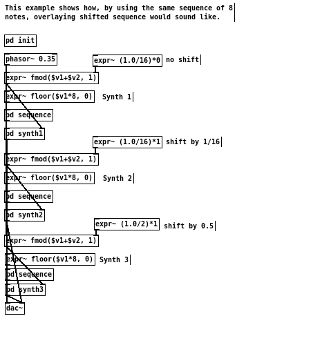
Musically speaking, it essentially adds a time delay/offset to the original control signal. One way this can be useful is to arrange the shifted signals in parallel, which would produce effects similar to a musical canon. In practice, this enables the ability to generate interesting compositional variations from a limited pre-defined sequence. Furthermore, the amount of shifting can also be modulated just the same way as amplitude and frequency, which allows for more dynamic and responsive structures to emerge.
For controlling sound synthesis, phase shifting provides a simple mechanism to move envelope and logic level along the time axis. Consider the following:
[phasor~ 0.25] -> [expr~ if($v1<0.25, 1, 0)] -> [s~ signal_1]
              \-> [expr~ fmod($v1+0.25, 1)] -> [expr~ if($v1<0.25, 1, 0)] -> [s~ signal_2]
signal_1 produces a gate switching signal with 25% duty cycle. By shifting the phase of the [phasor~], signal_2 would have the same rate of change, but delayed by quarter of the total wavelength.
It is worth mentioning that, attention needs to be paid to the total amount of shift that are “allowed”. that is to say, the “effective” shift permitted would be the total wave period minus the duty cycle of the gate. In the case of above example, if the amount of shift had been greater than 0.75, the “on” portion of the gate would be pushed off the right edge, and thus may cause undesired effect.
Exercise:
- How to shift the phase of a sine wave?
-*-
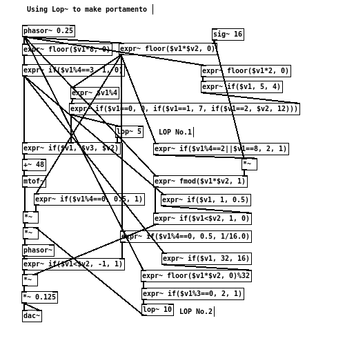
By default, functions such as floor() or if() would produce a “hard” stepped signal. That is to say, signal changes abruptly from one level to the next, governed by predefined functions and timing. Whilst this behaviour is absolutely expected and correct, it may not results to the most “musical” effect at times. In other words, being able to move seamlessly from one value to another can contributes to a more “natural” quality to the composition. Musically, such an effect can be seen as “portamento”, where by the pitch slides from note to note, rather than stepped.
A simple one-pole low pass filter can be used in this case to “smooth” out incoming signal, making it much less abrupt. consider the following:
[phasor~ 0.5] -> [expr~ (floor($v1*4, 0)+1)*200] -> [osc~] -> [dac~]
and
[phasor~ 0.5] -> [expr~ (floor($v1*4, 0)+1)*200] -> [lop~ 10] -> [osc~] -> [dac~]
The value 10 given as the argument to [lop~] specifies the filter’s cut-off frequency, and in this case, it translates to the time taken to smooth out the incoming signal. For example, 1Hz would equates to 1 second in time, whereas 10Hz would only take 100 millisecond.
It is also worth noting that if the frequency given to [lop~] is lower/slower than the rate of the main timing, the resulting signal may never fully reach its target value. In this case, it would simple wobble along between different values.
Another use case for [lop~] would be a quick-and-dirty envelop set-up, such as:
[phasor~ 1] -> [expr~ if($v1<0.5, 1, 0)] -> [lop~ 5]
Ordinarily, such type of “gate” switching would produce clicks at the edges of the on state. However, by passing the signal through a low pass filter, the hard edges thus are rounded off, making the transitions much less harsh.
The following example shows an simple riff using 2 [lop~]:
Exercise:
- Are there any other use case for [lop~]
- What are the drawback of the [lop~] object in Pd used in this context?
- How about using other types of filters?
-*-
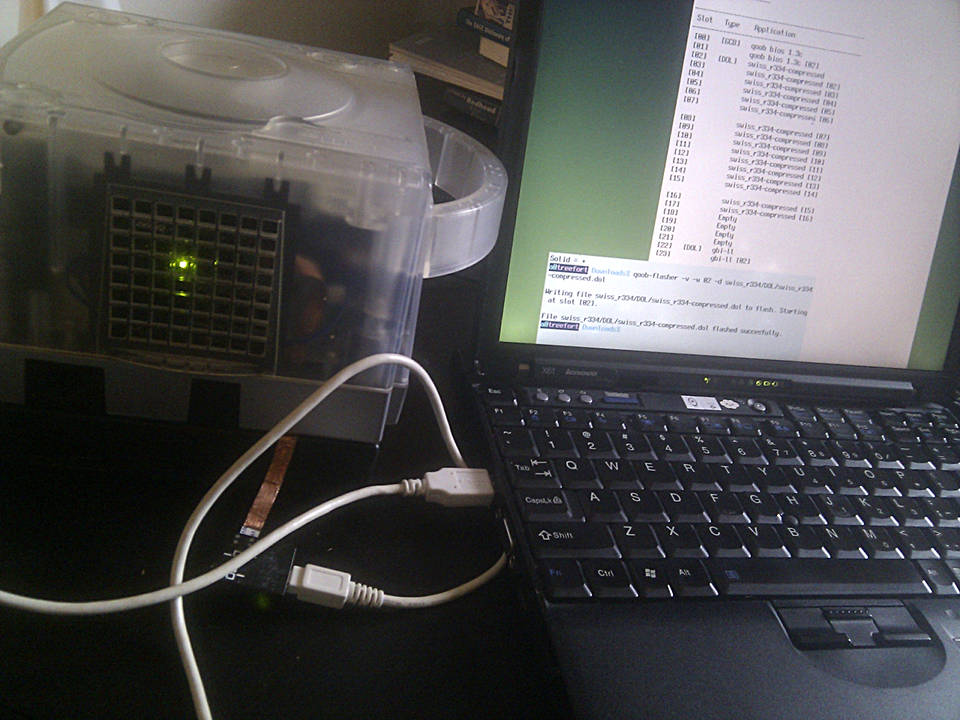
Sometimes ago I dug up my old GameCube to give a try to GBI, a very impressive homebrew alternative to the Game Boy Player Start-up Disc.
To load homebrews, the GC had been modded 10 years ago by someone with a now impossible to find Qoob Chip Pro. This great modchip was only provided with a Windows software to flash it. However while looking for a copy of the program, I stumbled upon a really nice Linux CLI version by Joni Valtanen. The software compiles and run fine on Debian, but I also wanted to have it available on FreeBSD. As it turns out, making it working for FreeBSD was fairly straightforward. Crappy patches below.
The flashing software comes in two parts: libqoob and qoob-flasher. Only libqoob sources need to be very slightly adjusted. FreeBSD comes with a specific libusb implementation, so there is no need to check for the regular one while configuring, but the libqoob pkg-config file needs to be edited to point to the libusb shipped with the OS. Also, pkg-config files are not located in a subdir of the lib directory on FreeBSD. All together, some changes need to be made to Makefile.am, configure.ac and libqoob.pc.in:
libqoob/Makefile.am:
diff --git a/libqoob/Makefile.am b/libqoob/Makefile.am
index 51cc260..7adacfb 100644
--- a/libqoob/Makefile.am
+++ b/libqoob/Makefile.am
@@ -7,7 +7,11 @@ all-local: $(pcfiles)
 %.pc: %.pc
        cp $< $@

+if FREEBSD
+pkgconfigdir = /usr/local/libdata/pkgconfig
+else
 pkgconfigdir = $(libdir)/pkgconfig
+endif
 pkgconfig_DATA = $(pcfiles)

 deb-install:
libqoob/configure.ac:
diff --git a/libqoob/configure.ac b/libqoob/configure.ac
index 0ff95f2..13a0df2 100644
--- a/libqoob/configure.ac
+++ b/libqoob/configure.ac
@@ -16,9 +16,18 @@ if test -z "$PKG_CONFIG" ; then
   AC_MSG_ERROR( pkg-config is required )
 fi

-PKG_CHECK_MODULES(libusb, [libusb >= 0.1.12], , AC_MSG_ERROR( libusb >= 0.1-12
is required ))
-AC_SUBST(libusb_CFLAGS)
-AC_SUBST(libusb_LIBS)
+if test "$(uname)" == "FreeBSD"; then
+  PKG_CHECK_MODULES(libusb, [libusb-0.1 >= 0.1], , AC_MSG_ERROR( libusb >= 0.1
is required ))
+  AC_SUBST(libusb_CFLAGS)
+  AC_SUBST(libusb_LIBS)
+  AC_SUBST(PACKAGE_REQUIRES, [libusb-0.1])
+  AM_CONDITIONAL([FREEBSD], [true])
+else
+  PKG_CHECK_MODULES(libusb, [libusb >= 0.1.12], , AC_MSG_ERROR( libusb >= 0.1-12 is required ))
+  AC_SUBST(libusb_CFLAGS)
+  AC_SUBST(libusb_LIBS)
+  AC_SUBST(PACKAGE_REQUIRES, [libusb])
+fi

 dnl debug
 AC_ARG_ENABLE(debug,
libqoob/libqoob.pc.in:
diff --git a/libqoob/libqoob.pc.in b/libqoob/libqoob.pc.in
index 027e026..559e77c 100644
--- a/libqoob/libqoob.pc.in
+++ b/libqoob/libqoob.pc.in
@@ -6,6 +6,6 @@ includedir=@includedir@/libqoob
 Name: libqoob
 Description: Qoob Pro flasher library
 Version: @VERSION@
-Requires: libusb
+Requires: @PACKAGE_REQUIRES@
 Libs: -L${libdir} -lqoob
 Cflags: -I${includedir}
Almost there. FreeBSD needs free() from its own memory allocation functions:
diff --git a/libqoob/src/qoob-defaults.h b/libqoob/src/qoob-defaults.h
index aa17409..116f2f1 100644
--- a/libqoob/src/qoob-defaults.h
+++ b/libqoob/src/qoob-defaults.h
@@ -20,6 +20,11 @@
 #ifndef _QOOB_DEFAULTS_H_
 #define _QOOB_DEFAULTS_H_

+#if defined(__FreeBSD__)
+#include <stdlib.h>
+#include <malloc_np.h>
+#endif
+
 /* Common typedefs */
 typedef enum {
   QOOB_FALSE = 0,
Now libqoob will compile and install fine, and qoob-flasher will configure, compile and install nicely out of the box on both Linux and FreeBSD.
It’s now time to plug your qoob’ed GC which will be claimed by the generic USB HID module:
ugen1.2: <QooB Team> at usbus1
uhid0: <QooB Team QOOB Chip Pro, class 0/0, rev 1.10/1.00, addr 2> on usbus1
However unlike on Linux, qoob-flasher will not be bothered by that, so there is a no need to blacklist the device! And now let’s flash some homebrew :)
-*-
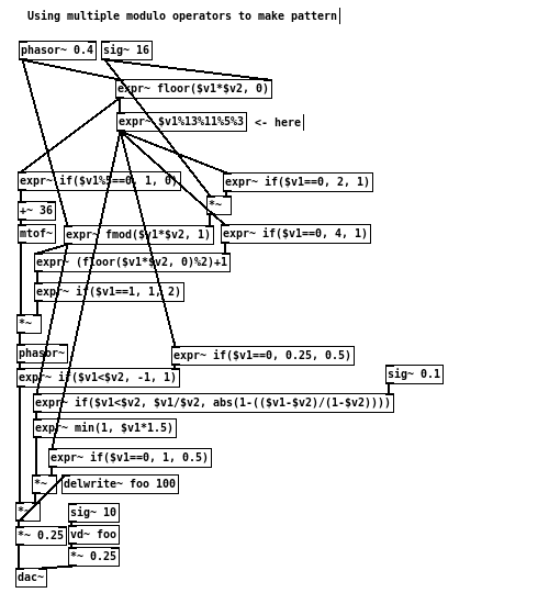
The modulo operator can be useful in making (pseudo) generative patterns. Not only its relatively easy to use, the process is also responsive to parameter changes. In other words, complex structures can be derived from simple operations, the transitions between perceivingly different patterns can also be quickly made.
The following two examples illustrates a simple usage of modulo and the resulting patterns:
if($v1%4 == 0, 1, 0):
COUNTER: 0 1 2 3 4 5 6 7 8 9 A B C D E F . . . .
PATTERN: 1 0 0 0 1 0 0 0 1 0 0 0 1 0 0 0 . . . .

if($v1%5 == 0, 1, 0):
COUNTER: 0 1 2 3 4 5 6 7 8 9 A B C D E F . . . .
PATTERN: 1 0 0 0 0 1 0 0 0 0 1 0 0 0 0 1 . . . .
Such implementation don’t produce interesting results by itself, unless the patterns are stacked/layered against each other.
However, by chaining modulo operators one after another, the result quickly becomes more complex. For example:
if(($v1%5)%3 == 0, 1, 0):
COUNTER: 0 1 2 3 4 5 6 7 8 9 A B C D E F . . . .
PATTERN: 1 0 0 1 0 1 0 0 1 0 1 0 0 1 0 1 . . . .

if((($v1%7)%4)%3 == 0, 1, 0):
COUNTER: 0 1 2 3 4 5 6 7 8 9 A B C D E F . . . .
PATTERN: 1 0 0 1 1 0 0 1 0 0 1 1 0 0 1 0 . . . .

if((($v1%11)%7)%4 == 0, 1, 0):
COUNTER: 0 1 2 3 4 5 6 7 8 9 A B C D E F . . . .
PATTERN: 1 0 0 0 1 0 0 1 0 0 0 1 0 0 0 1 . . . .
The general principle is thus to use progressively smaller values after each modulo operator, so to nest smaller counts inside of larger loops. Often, these divisors, especially towards smaller ones, can be modulated by other time measure, so to increase the diversity of the resulting pattern.
Furthermore, since largest divisor determines the length of the entire pattern, by modulating it would also produce different pattern, even if the rest of the expression remains the same. Consider the following:
if(($v1%5)%3 == 0, 1, 0) vs. if(($v1%7)%3 == 0, 1, 0):
COUNTER: 0 1 2 3 4 5 6 7 8 9 A B C D E F . . . .
PATTERN: 1 0 0 1 0 1 0 0 1 0 1 0 0 1 0 1 . . . .
PATTERN: 1 0 0 1 0 0 1 0 0 1 0 0 1 0 1 0 . . . .
Notice that the examples so far uniformly select the first count to give the final structure, but the following can also be considered:
if(($v1%5)%3 == $v2)
where $v2 is a modulated signal to select which element
in the count is to be used.
Here is an quick example using modulo operator to make Djent:)
Exercise:
- What other ways can modulo be useful to make/manipulate patterns?
- How to use phase shift to further process the resulting pattern?
-*-
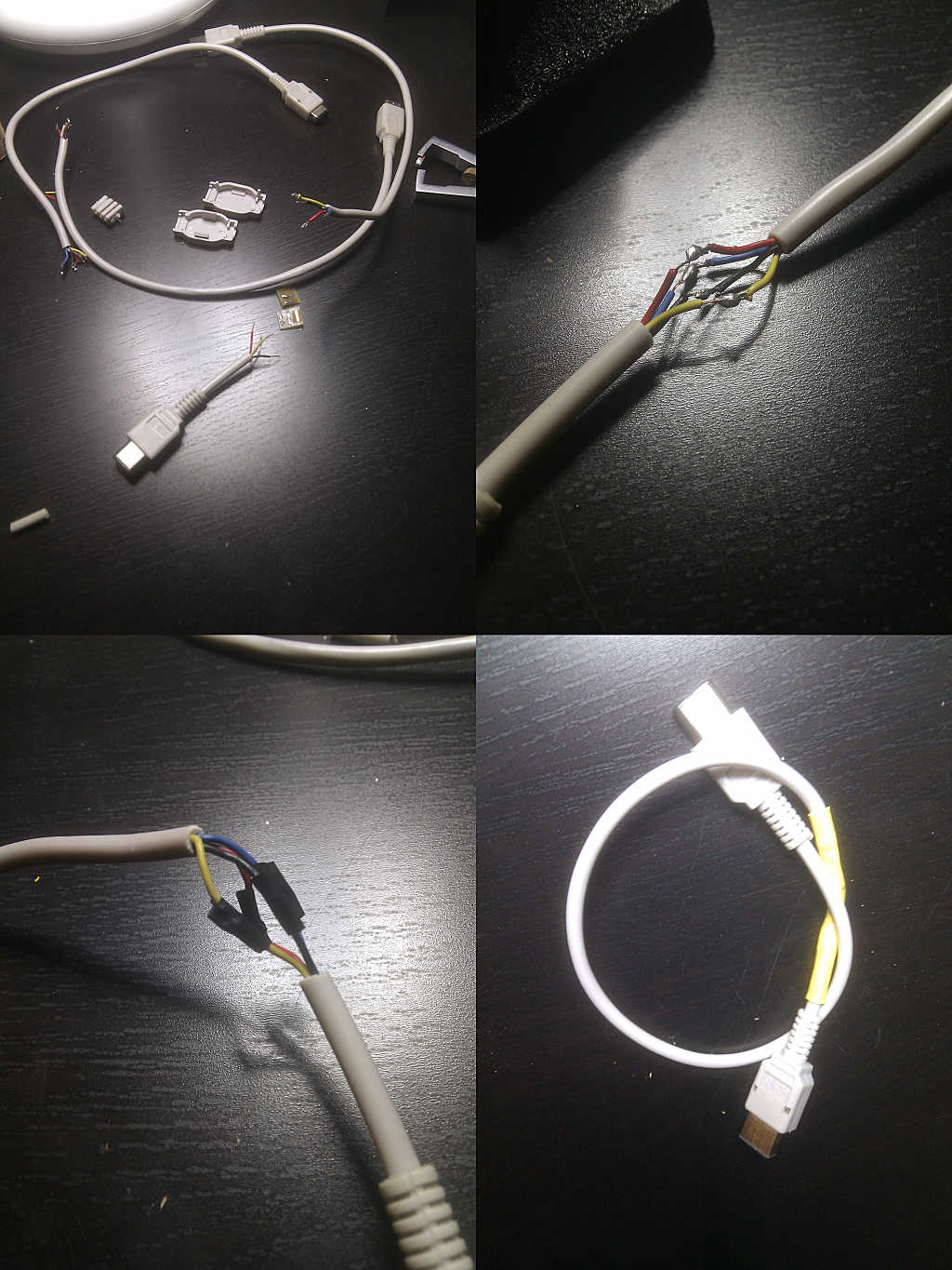
Can’t trade your pokémouille anymore?!
Fear not. Old GB link cables, specially third party, tend to eventually suffer from contact failure. Connectors are usually OK, but the wires not, which will give much headache if the link is used to transfer data (hello corrupted saved banks, hello wasted last night).
The fix is easy though, cut the defective parts and solder back the… possibly much shorter… new cable.
 ___________                       ___________
|  6     2  |---------------------|  6     2  |
 \_5__3____/                       \_5__3____/
 Connector 1                       Connector 2

Connector 1

2   SOUT  Data Out        Black
3   SIN   Data In         Blue
5   SCK   Shift Clock     Yellow
6   GND   Ground          Red

Connector 2
(may have data wires color reversed for optimised
assembly line slavery)

2   SOUT  Data Out        Blue (!)
3   SIN   Data In         Black (!)
5   SCK   Shift Clock     Yellow
6   GND   Ground          Red

 SOUT ---------- SIN
 SIN  ---------- SOUT
 SCK  ---------- SCK
 GND  ---------- GND
Here is a dodgy 4 plugs GB/GBC link turned into a working 2 plugs GB link.
-*-
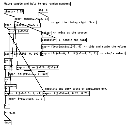
Having random values are often a quick and easy method to create variations in compositional arrangements. Conventionally, the [random] object is used for this purpose. By triggering the object with a bang, it would output a new value within a specifiable range.
Random values can also be obtained using only audio control signals, which involves the use of sample and hold function ([samphold~] in Pd). Generally speaking, it takes a snapshot of its input/source signal, and output the sample value until it samples again. The second inlet of [samphold~], therefore, controls how often the new samples are taken. In this case, it is when the signal to the second inlet has a negative transition/increment.
For example, if a [phasor~] is connected to the second input, [samphold~] will be triggered right at the boundary between each wave cycle. This is because only at that point, the increment of [phasor~] would be negative. This unique property of sawtooth wave enables [samphold~] to take one-off samples at regular interval.
Once the principle of [samphold~] is understood, simply connecting a [noise~] object to its first input would result to a randomized signal. The random values would consequently change according to the signal characteristics given to the second inlet. Simple numerical manipulation might be necessary in order to scale the values to a appropriate range thereafter.
Exercise:
- Besides using [noise~] as a source for randomised signal, what other use might [samphold~] also have?
- What other wave forms might also be interesting to be used as the control signal for [samphold~]?
-*-
Modulation, sequencing, division of time unit are simple ways to utilise a (Sawtooth) signal in order to achieve certain functions. How in which they are put together therefore determines the “arrangement” of the composition.
One simple approach in combining these elementary components, is to deduce the possibilities into two basic types: serial and parallel.
Serial, implies putting these functions one after another, so to produce desired outcome at the end of the chain. It typically results to control signals for modulation, or for logic control. The intermediate steps, in this case, involves resolving the correct timing frequency. In the example below, the fmod() is first used to divide the wave period of the incoming sawtooth, and then passed onto the next [expr~] to produce triangle wave.
[phasor~ ]->[expr~ fmod($v1*4, 1)]->[expr~ abs(abs($v1-0.5)-0.5)*2]
Parallel, on the other hand, refers to the diverging of signals, so that branches are created with each of the strand serving a different purpose. A common usage of this set-up would be to control various aspects of a given sound synthesis algorithm, from within a same time scope. For example, by using fmod() and floor() from the same timing signal, one can produce amplitude envelopes, as well as counters to alter the frequency of an oscillator at the same time. This process is very much the same as how control voltage (CV) is used in analog synthesiser.
   [phasor~ ]->[expr~ fmod($v1*4, 1)]->[expr~ abs(abs($v1-0.5)-0.5)*2]->[send~ amp_env]
             \ ->[expr~ floor($v1*4, 0)]->[expr~ if($v1%2, 2,1)]->[send~ freq]
As seen in above examples, serial connections are generally not very long, unless multiple steps are taken to derive the necessary timing. By grouping multiple serial process, a parallel arrangement is thus formed. Moreover, different group of parallel process can also be interconnected in a serial fashion, so to manipulate the composition at different scope of time.
In short, such a generalisation are guide lines in which can be used as a starting point when applying these techniques in composition. One other useful way in approaching the subject would be seeing it essentially the same as how CV signals are used analogue modular synthesiser.
Exercise:
- Using the example patch, extend it into a 4 bar phrase.
- Using the example patch, make other voice/concurrent parts in the arrangement.
-*-